|
Its been a long time coming, but I finally got around to implementing sub-sampling U,V in the JPEG writer. This means many files are 20-30% smaller than before with very little visual quality loss. Sub-sampled UV is enabled automatically for quality levels <= 90. The new code functions exactly like it did before with the same API as before. Drop it in and enjoy!
0 Comments
Oodle Lossless Image (OLI) version 1.4.7 was just released. In this release there is lots of improvements - specifically with palettized and 1/2 component images. Also in 1.4.7 is a basic Unity engine integration! OLI now supports palettized images -- up to 2048 unique colors (though it could go as high as 64k, but I didn't see a benefit in my test set to go higher than 2048). Implementing this was pretty interesting in that the order of those colors in the palette matter quite a bit - and the reason is that if you get it right, then it works with the prediction filters. As in, if the palettized color indexes are linearly predictable then there is a good chance you will get significantly better compression than just a random ordering. In practice this means trying a bunch of different heuristics (since computing optimal brute force like is prohibitively expensive). So you sort by luma, or by different channels, or by distance from the last color for example (picking the most common color as the first one). I also implemented mZeng palette ordering technique which isn't commonly in PNG compressors. Believe it or not, while this theoretically should produce really good results in most cases, sometimes the simpler heuristics win by a lot so you can't just always use a single method to decide when going for minimum file sizes. Examples (some images I've seen used as examples on other sites): In all cases, the following arguments were used
pngcrush -brute <input> <output> cwebp -q 100 -lossless -exact -m 6 -mt <input> -o <output> flif -E100 -K <input> <output> Note that insane sometimes doing slightly worse than super-duper happens sometimes due to layered processes - just on average insane is going to be better. 1/2 Component images were just a matter of writing all the various SIMD routines to decode them. Other than that nothing special here except having fewer components means smaller files and faster decoding. I may in the future support more than 4 components if there is a demand for that, but for now its 1,2,3 or 4 components of 8 or 16-bits per component. There also were some general small encoding improvements. And soon coming up are some new color spaces which should further reduce file size. Specifically the new encoding flag called "--insane" which actually compresses stuff instead of using heuristics in most places to find whats the best thing to do. I use this for dev, but it might be useful for people looking to squeeze out a few more percent in file sizes. For more information on Oodle Lossless Image visit http://www.radgametools.com/oodlelimage.htm Note: This is a work-in-progress and still being tested for possible distribution issues. I will update this blog post as the work progresses. Trying to simplify my life a bit over here, I am on a journey to eliminate my Mac from the build iteration cycle. The goal is to completely ship all binaries for both Bink and Oodle Lossless Image (OLI) directly from my PC rather than occasionally building on a mac only to find that Apple broke yet another thing in the latest OSX update or iSDK release (seriously, stop that!). First thing first, your gonna need a toolchain. I used the toolchain from http://www.pmbaty.com/iosbuildenv/ which is claimed to be a native port of the apple tools opensource.apple.com/tarballs/. I also used MSys (via http://mingw.org/) over here so I could have my same build scripts that work on OSX work nearly transparently on Win as well with very little modification. To build for OSX, iOS, tvOS and watchOS you are going to need some sysroots from a real mac. You can find these and some frameworks you are going to need in each SDK release at the following paths
Next use clang to build for Apple by specifying some additional parameters. The first of which is your target specification.
Second, specify your framework directory. This is located in your {SDK}/System/Library/Frameworks directory, so would be specified as "-F{SDK}/System/Library/Frameworks" Third, you need to specify your sysroot as "--sysroot {SDK}". The sysroot tells the compiler where your headers and libs are. That's about it for building stuff (I think?). Just use as normal. To make a DMG file you need to do things a bit differently since there is no hdiutil on windows as it is closed-source apple tech. Instead of hdiutil, you use mkisofs (you can get that with mingw, or provided also right here...
invocation would look something like
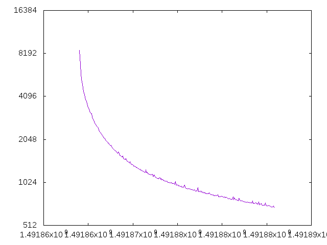
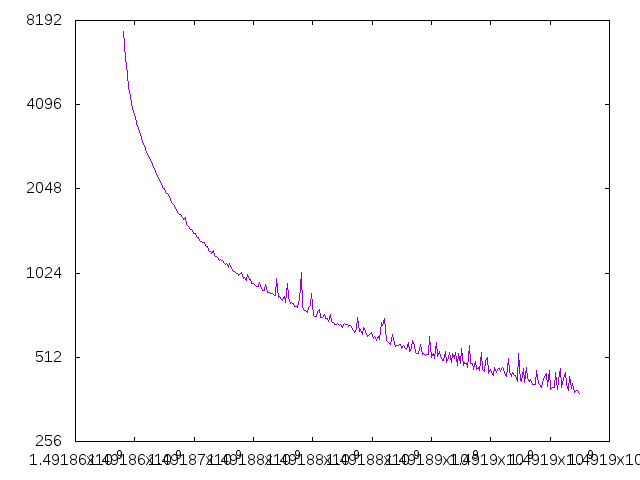
mkisofs -J -R -o {file}.dmg -mac-name -V "{title}" -apple -v -dir-mode 777 -file-mode 777 {dmg_directory} As for signing executables, I haven't yet had to worry about that... hoping I won't! I would point you to the pmbaty ios tools which has an executable signer in there. If I missed anything, or something is not clear or not working for you, please let me know in the comments below and I'll help if I can! A quick post about the results for my first comparison here of a 2-layer fully connected network vs a DagNN. I've removed most of the random variables here for this example so that the comparison is pretty accurate. The only random variable left is the order in which things are trained due to SGD - however, as I removed more and more random variables the differences got more in favor of DagNN and not less. The conclusion of this test is that DagNN is better node-for-node per epoch than the standard 2-layer fully connected network - at least in this example. This at least follows intuition a bit, that more weights between the same number of nodes increases overall computational power of the network.
More rigorous comparisons in some of the standard test cases needs to be done, but this is a good first step offering some preliminary credibility. I had an idea the other day while reading a paper about how they passed residuals around layers to keep the gradient going for really deep networks - to help alleviate the vanishing gradient issue. Then it occurred to me, perhaps that this splitting of networks into layers is not the best way to go about it. After all, the brain isn't organized into strict layers of convolution, pooling, etc... So perhaps this is us humans trying to force structure onto an unstructured task. Thus the DagNN was born over last weekend. Directed Acyclic Graph Neural Networks or DagNN for short.
First, a quick description of why/how many Deep Neural Networks are trained today as I understand it. The vanishing gradient problem is a problem to neural networks that arise because of how back-propagation works. You take the difference between the output of a network and the desired output of a network and then take the derivative of that node and pass that back through the network weighted by the connections. Then repeat for those connections on the next layer up. So you are passing a derivative of a derivative for 1 hidden layer networks and a derivative of a derivative of a derivative for 2 layer networks and so on. These numbers get "vanishingly" small very quickly - so much so that typically you tend to get *worse* results with a network with 3 or more layers vs just 1 or 2. So, how do you train "deep" networks with many layers? Typically with unsupervised pre-training, typically with an auto-encoder. An auto-encoder is when you train a network, 1 layer at a time stacking on top of each other with no specific training goal other than to reproduce the input. Each time you add a layer you lock the weights of the prior layer. This means your training a generic many layer network to just "understand" images in general as a combination of layered patterns rather than to solve any particular task. Which is better than nothing, but certainly not as good as if you could actually train the *entire* network to solve a specific task (intuitively). The solution: If you could somehow pass the gradient further down into the network, then you can train it "deeper" to solve specific tasks. Back to DagNNs. The basic premise follows the idea that if you pass the gradient further down the network, then you can train deeper networks to solve specific tasks. Win! But how? Simple, remove the whole concept of layers and just connect every node with every prior node allowing any computation to build on any other prior computation to solve the output. This means that the gradient filters through the entire network from the output in fewer hops. The way I like to think about DagNNs is the small world phenomenon. Or the degrees of kevin bacon if you prefer. You want your network to be able to get to useful information in 2-3 hops or the gradient tends to vanish. Pro tip: if you want to bound computational complexity, limit it to a random N number of prior connections per node. I'm trying out this idea now and at least initially it is showing promise. I can now train far bigger fully connected networks than I could before. Will release source when I have more proof in the pudding. By proof that means proof for me too! I need to train it on MNist and compare results. Just a quick post about the new 1.02 release of jo_mpeg.cpp In this update the color space was fixed to be more accurate. (Thanks for r- lyeh for reporting this bug!) Also, fixing the above uncovered a different issue in the AC encoding code, now fixed as well. END OF LINE
Neural Networks offer great promise with their ability to "create" algorithms to solve problems - without the programmer knowing how to solve the problem in the first place. Example based problem solving if you will. I would expect that if you knew precisely how to solve a particular problem to the same degree, you could certainly do it perhaps many orders of magnitude faster and possibly higher quality by coding the solution directly -- however its not always easy or practical to know such a solution.
One opportunity with NNs that I find most interesting is that, no matter how slow they are, you can use NNs as a kind of existence proof -- does an algorithm exist to solve this problem at all? Of course, when I'm talking about "problems" I'm referring to input to output mappings via some generic algorithm or something. Not everything cleanly fits into this definition, but many things do. Of course there are many different kind of NNs for solving various different kinds of problems too. After working with NNs for a while (and indeed to anybody who has) I can say that Neural Networks are asymmetric in complexity. That is, training a neural network to accomplish a task can take extreme amounts of time (days is common). However, executing a previously trained Neural Network is embarrassingly parallel and is pretty well mapped to GPUs. Running a NN can be done in real-time if the network is simple enough! I have spent considerable amounts of time in figuring out how to train Neural Networks faster. The generally recommended practice these days is to use Stochastic Gradient Descent (SGD) with Back Propagation (BP). What this means is you take a random piece of data out of your training set to train with, train with it, and then repeat. SGD works, but is *incredibly* slow at converging. I endeavored to improve the training performance here (how could you not, you spend a *lot* of time waiting...) There are many different techniques to improve upon BP (Adam, etc.. etc..), however each of them are in my measurements slower, regardless of the steeper descent they provide, they take more computation to provide that steeper descent and so when you measure not by epoch but by wall clock time, its actually slower. So, then came the theory that if you somehow knew the precise order to train the samples in, you could perfectly train to the correct solution in some minimum amount of time. I don't know if there is a theorem about this or what-not, but if not you now have heard of it. It seemed common sense to me. In any case, then the question becomes is there a heuristic which can approximate this theoretical "perfect" ordering? The first thing I tried turned out to be very hard to beat, calculate error on all samples, then sort the training order by the error for each in decreasing order. Then, only train 25% of the worst error samples. The speedup from this approach was pretty awesome, but again I got bored waiting so I went further. Essentially you don't waste time training the easy stuff and instead concentrate on learning the parts it has problems with. I then tried doing many variations on this, but the one that ended up working even better (30% improved training time) was taking the sorted order and splitting it into 3 sections of easy, medium and hard. Then reorganizing the training order into hard, medium, easy, hard, medium, easy, hard, medium, easy, etc... Not only did this improve the training time - it also was able to train to an overall lower error than without. Another option that works pretty well is to just take the 25% highest error samples and randomize the order. Its easier to implement and also works really well. Also, this should be overall a better approach (vs unrandomized) as it seems more robust to training situations where the error explodes (which does happen in some cases). Thats generally how I would approach a finite and small-ish data set. I am also developing a technique based on this that works for significantly larger data sets - ones that cannot possibly fit in memory (hundreds or thousands of images). Thus far the setup is fairly similar, except you pick some small batch of images and do basically the same as above with that. There are some interesting relationships between batch size (number of images) and training time/quality. In my data set, the size of the batch reduces the variance of the solution error across the training set and also appears thus far to reduce the number of epochs required to converge - however it is also slower so the jury is still out on if a bigger batch is better - but certainly going too small makes it harder to converge on a general solution. Thats all for now!
In this series of blog posts, I'm going to cover various parts of the research and development behind Bink 2 HDR.
There are 4 different color standards, namely Rec.601, Rec.709, Rec.2020, and Rec.2100. Rec.601, Rec.709 and Rec.2020 all have different definitions of R,G and B. Rec.2020 notably defines a "wide color gamut". Rec.2100 has the same color gamut as Rec.2020, but defines Percentual Quantiers (PQ) and Hybrid Log-Gamma (HLG) for UHDR. First, when working with HDR color spaces, be sure to use linear RGB inputs. No sRGB, Adobe RGB, etc... What about if your loading a floating point format like EXR or HDR? These are both linear, so no conversion *should* be necessary. There are three color spaces in Rec.2100.
Non-Constant Luminance (NCL) YCbCr
This color space is very similar to LDR YCbCr after tone mapping from 10k Luma to LDR range.
The code for converting to/from linear RGB to NCL Y'Cb'Cr' is as follows...
void RGBtoYCbCr2100(float *rgbx, float *ycbcr, int num) {
    for(int i = 0; i < num*4; i+=4) {
        float r = rgbx[i+0], g = rgbx[i+1], b = rgbx[i+2];
        r = smpte2084_encodef(r);
        g = smpte2084_encodef(g);
        b = smpte2084_encodef(b);
        ycbcr[i+0] = 0.2627f*r + 0.6780f*g + 0.0593f*b;
        ycbcr[i+1] = -0.13963f*r - 0.36037f*g + 0.5f*b;
        ycbcr[i+2] = 0.5f*r - 0.45979f*g - 0.040214f*b;
        ycbcr[i+3] = rgbx[i+3];
    }
}

void YCbCrtoRGB2100(float *ycbcrx, float *rgbx, int num) {
    for(int i = 0; i < num*4; i+=4) {
        float Y = ycbcrx[i+0], Cb = ycbcrx[i+1], Cr = ycbcrx[i+2];
        float r = Y + 1.4746f*Cr;
        float g = Y - 0.164552f*Cb - 0.571352f*Cr;
        float b = Y + 1.8814f*Cb;
        r = smpte2084_decodef(r);
        g = smpte2084_decodef(g);
        b = smpte2084_decodef(b);
        rgbx[i+0] = r;
        rgbx[i+1] = g;
        rgbx[i+2] = b;
        rgbx[i+3] = ycbcrx[i+3];
    }
}
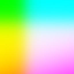
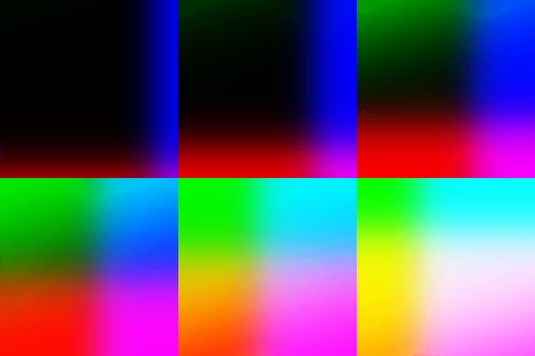
We can display these color spaces using LDR images via tone mapping - as shown below.
Constant Luminance ICtCp
Rec.2100, the latest standard, defines a new color space for HDR which improves on the NCL & CL YCbCr called ICtCp.
The code for converting from Rec.2020 linear RGB to ICtCp is as follows...
void RGBtoICtCp(float *rgbx, float *ictcpx, int num) {
    for(int i = 0; i < num*4; i+=4) {
        double r = rgbx[i+0], g = rgbx[i+1], b = rgbx[i+2];
        double L = 0.4121093750000000*r + 0.5239257812500000*g + 0.0639648437500000*b;
        double M = 0.1667480468750000*r + 0.7204589843750000*g + 0.1127929687500000*b;
        double S = 0.0241699218750000*r + 0.0754394531250000*g + 0.9003906250000000*b;
        L = smpte2084_encodef(L);
        M = smpte2084_encodef(M);
        S = smpte2084_encodef(S);
        ictcpx[i+0] = 0.5*L + 0.5*M;
        ictcpx[i+1] = 1.613769531250000*L - 3.323486328125000*M + 1.709716796875000*S;
        ictcpx[i+2] = 4.378173828125000*L - 4.245605468750000*M - 0.132568359375000*S;
        ictcpx[i+3] = rgbx[i+3];
    }
}
The inverse transform of ICtCp back to Rec.2020 RGB is as follows:
void ICtCptoRGB(float *ictcpx, float *rgbx, int num) {
    for(int i = 0; i < num*4; i+=4) {
        double I = ictcpx[i+0], T = ictcpx[i+1], P = ictcpx[i+2];
        double L = I + 0.00860903703793281*T + 0.11102962500302593*P;
        double M = I - 0.00860903703793281*T - 0.11102962500302593*P;
        double S = I + 0.56003133571067909*T - 0.32062717498731880*P;
        L = smpte2084_decodef(L);
        M = smpte2084_decodef(M);
        S = smpte2084_decodef(S);
        rgbx[i+0] =  3.4366066943330793*L - 2.5064521186562705*M + 0.0698454243231915*S;
        rgbx[i+1] = -0.7913295555989289*L + 1.9836004517922909*M - 0.1922708961933620*S;
        rgbx[i+2] = -0.0259498996905927*L - 0.0989137147117265*M + 1.1248636144023192*S;
        rgbx[i+3] = ictcpx[i+3];
    }
}
ICtCp claims that it provides an improved color representation that is designed for high dynamic range (HDR) and wide color gamut (WCG). It also claims that for CIEDE2000 color quantization errors 10-bit ICtCp would be equal to 11.5 bit YCbCr. Constant luminance is also improved with ICtCp which has a luminance relationship of 0.998 between the luma and encoded brightness while YCbCr has a luminance relationship of 0.819. An improved constant luminance is an advantage for color processing operations such as chroma subsampling and gamut mapping where only color information is changed.
Note, that I haven't verified these claims yet... Again, here is this color space converted to LDR via tone mapping. Evaluation of Color Spaces
To evaluate the color spaces, I am looking for a few different properties (that come to mind)
Additional Snippets
static double smpte2084_decodef(double fv) {
    double num, denom;
    fv = pow(fv, 1/SMPTE_2084_M2);
    num = fv - SMPTE_2084_C1;
    num = num < 0 ? 0 : num;
    denom = SMPTE_2084_C2 - SMPTE_2084_C3 * fv;
    return pow(num / denom, 1/SMPTE_2084_M1);
}

static double smpte2084_encodef(double v) {
    double tmp = pow(v, SMPTE_2084_M1);
    return pow((SMPTE_2084_C1 + SMPTE_2084_C2 * tmp) / (1 + SMPTE_2084_C3 * tmp), SMPTE_2084_M2);
}
References
Probably others, but these are the important ones.
In this series of blog posts, I'm going to cover various parts of the research and development behind Bink 2 HDR.
So first thing is deciding on an encoding. Of which there are a very many to choose from. There is...
Just to name a few. Additionally with video games, we have additional constraints such as texture filtering and performance considerations, etc... For example, bi-linear filtering is a linear operation, and the luma representation would have to operate correctly under linear transforms (or at least be fast enough to decode so that it wouldn't matter to first decode then interpolate). Additional x 2 for a video format like Bink, we need to consider various compression artifacts and what those would look like. With so many different formats to choose from, you have to take a step back and instead look at the actual encoding used by the output itself - as that really determines what is best (or used directly). Which leads me to the next topic of SMPTE 2084. SMPTE-2084 ... aka High Dynamic Range Electro-Optical Transfer Function of Mastering Reference Displays (try saying that 5 times fast!) SMPTE-2084 is the format to which Dolby Vision and HDR10 displays use - so its basically the narrow part of the pipeline. Everything you want to display has to go through this non-linear encoding at some point before being displayed on the TV (decoded back to linear in the process as well). The SMPTE-2084 format is locked behind a pay wall (yay) - which I have purchased and will boil it down for you to what I believe is the most important parts. The format defines luma in absolute values between 0 to 10,000 cd/m^2 (candelas per square meter). However, with the caveat that in real implementations of the spec, 10k luma won't actually be representable in anything but pure white color. Additionally, actual displays vary from the absolute curve due to output limitations and effects of non-ideal viewing environments. While the format supports 10, 12, 14, and 16-bit Luma representations, as currently deployed Dolby Vision is 12-bit and HDR10 is 10-bit. 14 and 16-bit is not widely deployed - if deployed at all anywhere other than the reference monitor. Additionally, these are positive numbers only. No negative values. The code to encode/decode a SMPTE-2084 is as follows.
#define SMPTE_2084_M1 (2610.f/4096*0.25f)
#define SMPTE_2084_M2 (2523.f/4096*128)
#define SMPTE_2084_C1 (3424.f/4096)
#define SMPTE_2084_C2 (2413.f/4096*32)
#define SMPTE_2084_C3 (2392.f/4096*32)

// Gives a value of 0 .. 10,000 in linear absolute brightness
float smpte2084_decode(unsigned v, int bits) {
    float fv, num, denom;
    fv = v / ((1 << bits)-1.f);
    fv = fv > 1.f ? 1.f : fv; // Clamp 0 .. 1
    fv = powf(fv, 1.f/SMPTE_2084_M2);
    num = fv - SMPTE_2084_C1;
    num = num < 0.f ? 0.f : num;
    denom = SMPTE_2084_C2 - SMPTE_2084_C3 * fv;
    return powf(num / denom, 1.f/SMPTE_2084_M1) * 10000.f;
}

// Gives a value between 0 and 2^bits-1 (non-linear)
unsigned smpte2084_encode(float v, int bits) {
    float n, tmp;
    v /= 10000.f;
    v = v > 1.f ? 1.f : v < 0.f ? 0.f : v; // Clamp 0 .. 1
    tmp = powf(v, SMPTE_2084_M1);
    n = powf((SMPTE_2084_C1 + SMPTE_2084_C2 * tmp) / (1 + SMPTE_2084_C3 * tmp), SMPTE_2084_M2);
    return (int)floorf(((1 << bits)-1) * n + 0.5f);
}
The pretty nice thing about the limited range here (10 to 12 bits) is that you can pre-generate a table to decode into floats and store it in a texture or constant buffer or whatever. This makes decoding rather inexpensive! There are still some open questions here regarding its suitability as a video encoding format that I have. Namely...
To be continued.... Announcing my STB style 256 lines of code MPEG1/2 writer! In this initial release the features are: 1) 256 lines of C code (single file) 2) no memory allocations 3) public domain 4) patent free (as far as I know) There is a lot left to be done, notably the encoding of P frames and audio. However, this is very useful as is for a drop-in MPEG writer in any project. Basic Usage: FILE *fp = fopen("foo.mpg", "wb"); jo_write_mpeg(fp, frame0_rgbx, width, height, 60); jo_write_mpeg(fp, frame1_rgbx, width, height, 60); jo_write_mpeg(fp, frame2_rgbx, width, height, 60); // ... fclose(fp); Some notes that this writer takes advantage of the fact that MPEG1/2 is designed so that you can literally concatenate files together to combine movies. Technically each frame is its own movie (until p-frames are implemented, then a set of frames would be its own movie). Some video players mess up here and don't decode correctly, but MPlayer, SMPlayer, FFMpeg and others work correctly. So this is great as a quick intermediate format! Have fun and code responsibly! (j/k)
|
Archives
November 2021
Categories |
||||||||||||||||||||||||||||||||||||||||||||||||||||||||||||



 RSS Feed